How to solve an equation in Excel. Finding a MS EXCEL solution

The Solver Excel add-in is an analytical tool that allows us to quickly and easily determine when and what result we will get under certain conditions. The capabilities of the solution search tool are much higher than what “parameter selection” in Excel can provide.

The main differences between finding a solution and selecting a parameter:

Selecting several parameters in Excel.
Imposing conditions to limit changes in cells that contain variable values.
Possibility of use in cases where there may be many solutions to one problem.

Examples and problems to find solutions in Excel

Let's look at the analytical capabilities of the add-in. For example, you need to save $14,000 in 10 years. For 10 years, you want to put $1,000 into a bank deposit account every year at 5% per annum. The figure below contains a table in Excel, which clearly shows the balance of accumulated funds for each year. As can be seen, under such conditions of a deposit account and savings contributions, the goal will not be achieved even after 10 years. When solving this problem, you can go in two ways:

Find a bank that offers a higher interest rate on deposits.
Increase the amount of annual savings contributions to your bank account.

We can change the variable values in cells B1 and B2 so as to select the necessary conditions for accumulating the required amount of money.

The “Solution Search” add-on allows us to simultaneously use 2 of these options to quickly simulate the most optimal conditions for achieving the goal. To do this:

As you can see, the program slightly increased the interest rate and the amount of annual contributions.

Limiting parameters when searching for solutions

Let's say you go to the bank with this table, but the bank refuses to raise your interest rate. In such cases, we need to find out how much we will have to increase the amount of annual investments. We must set a cell constraint with one variable value. But before you start, change the values in the variable cells to the original ones: in B1 by 5%, and in B2 by -$1000. Now let's do the following.

In this article you will learn how solve quadratic equation inExcel on a specific example. Let us analyze in detail the solution to a simple problem with pictures.

Progress of the decision

Let's launch Microsoft Office Excel. I'm using the 2007 version. First, let's combine cells A1:A5 and write the quadratic formula in them in the form ax2+bx+c=0. Next, we need to square x, to do this we need to make the number 2 a superscript. Select the two and right-click.

We get a formula of the form ax 2 +bx+c=0

In cell A2 we enter the text value a=, in cell A3 b= and in cell A4 c=, respectively. These values will be entered from the keyboard in the following cells (B2,B3,B4).

Let's enter text for the values that will be calculated. In cell C2 d=, C3 x 1 = C4 x 2 =. Let's make the sublinear spacing for x similar to the superscript spacing in x 2

Let's move on to entering formulas for the solution

The discriminant of a quadratic trinomial is b 2 -4ac

In cell D2, enter the appropriate formula for raising a number to the second power:

A quadratic equation has two roots if the discriminant is greater than zero. In cell C3, enter the formula for x 1

IF(D2>0;(-B3+ROOT(D2))/(2*B2);”No roots”)

To calculate x2, we introduce a similar formula, but with a plus sign

IF(D2>0;(-B3-ROOT(D2))/(2*B2);”No roots”)

Accordingly, with the entered values a, b, c, the discriminant is first calculated, if its values are less than zero, the message “No roots” is displayed, otherwise we get the values x 1 and x 2.

Protecting a sheet in Excel

We need to protect the sheet on which we made the calculations. Without protection, you need to leave cells in which you can enter values a, b, c, that is, cells B2 B3 B4. To do this, select this range and go to the cell format, go to the Reviews tab, Protect Sheet and uncheck the Protected cell box. Click OK to confirm the changes made.

This range of cells will not be protected when the worksheet is protected. Let's protect the sheet; to do this, go to the Review tab and select Sheet Protection. Let's enter the password 1234. Click OK.

Now we can change the values of cells B2,B3,B4. When we try to change other cells, we will receive the following message: “The cell or chart is protected from changes. And also advice on removing protection.

You may also be interested in the material on how to secure it.

Excel has a wide range of tools for solving different types of equations using different methods.

Let's look at some solutions using examples.

Solving equations by selecting Excel parameters

The Parameter Selection tool is used in a situation where the result is known, but the arguments are unknown. Excel adjusts the values until the calculation gives the desired total.

Path to the command: “Data” - “Working with data” - “What-if analysis” - “Parameter selection”.

Let's look at the example of solving the quadratic equation x 2 + 3x + 2 = 0. The procedure for finding the root using Excel:

The program uses a cyclic process to select a parameter. To change the number of iterations and error, you need to go to the Excel options. On the “Formulas” tab, set the maximum number of iterations and relative error. Check the “enable iterative calculations” checkbox.

How to solve a system of equations using the matrix method in Excel

The system of equations is given:

The roots of the equations are obtained.

Solving a system of equations using the Cramer method in Excel

Let's take the system of equations from the previous example:

To solve them using Cramer's method, we calculate the determinants of the matrices obtained by replacing one column in matrix A with the column-matrix B.

To calculate the determinants, we use the MOPRED function. The argument is a range with the corresponding matrix.

Let's also calculate the determinant of matrix A (array - range of matrix A).

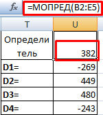
The determinant of the system is greater than 0 – the solution can be found using Cramer’s formula (D x / |A|).

To calculate X 1: =U2/$U$1, where U2 – D1. To calculate X 2: =U3/$U$1. Etc. Let's get the roots of the equations:

Solving systems of equations using the Gaussian method in Excel

For example, let’s take the simplest system of equations:

3a + 2b – 5c = -1
2a – b – 3c = 13
a + 2b – c = 9

We write the coefficients in matrix A. Free terms - in matrix B.

For clarity, we highlight the free terms by filling. If the first cell of matrix A contains 0, you need to swap the rows so that a value other than 0 appears here.

Examples of solving equations using the iteration method in Excel

The calculations in the workbook should be set up as follows:

This is done on the “Formulas” tab in “Excel Options”. Let's find the root of the equation x – x 3 + 1 = 0 (a = 1, b = 2) by iteration using cyclic references. Formula:

Х n+1 = X n – F (X n) / M, n = 0, 1, 2, … .

M – maximum value of the modulo derivative. To find M, let's do the calculations:

f’ (1) = -2 * f’ (2) = -11.

The resulting value is less than 0. Therefore, the function will have the opposite sign: f (x) = -x + x 3 – 1. M = 11.

In cell A3 we enter the value: a = 1. Accuracy – three decimal places. To calculate the current value of x in the adjacent cell (B3), enter the formula: =IF(B3=0;A3;B3-(-B3+POWER(B3;3)-1/11)).

In cell C3, let's control the value of f (x): using the formula =B3-POWER(B3,3)+1.

The root of the equation is 1.179. Let's enter the value 2 into cell A3. We get the same result:

There is only one root on a given interval.

There are many problems that can be significantly easier to solve using the Solution Finder tool. But to do this, you need to start by organizing the worksheet according to a model suitable for finding solutions, which requires a good understanding of the relationships between variables and formulas. Although the formulation of the problem usually presents the main difficulty, the time and effort spent on preparing the model are fully justified, since the results obtained can protect against unnecessary waste of resources, in case of incorrect planning, help increase profits through optimal financial management or identify the best ratio of production volumes, inventories and product names.

Behind your essence optimization problem is a mathematical model of a certain process of product production, its distribution, storage, processing, transportation, purchase or sale, performance of a range of services, etc. This is a common math problem of the Given/Find/Condition type, but which has many possible solutions. Thus, the optimization problem is the task of choosing from many possible options the best, optimal one. The solution to such a problem is called plan or program, for example, they say - a production plan or a reconstruction program. In other words, these are the unknowns that we need to find, for example, the amount of production that will give the maximum profit. The optimization problem is the search for an extremum, that is, the maximum or minimum value of a certain function, which is called target function For example, this could be a profit function - revenue minus costs. Since everything in the world is limited (time, money, natural and human resources), optimization problems always have certain restrictions, for example, the amount of metal, workers and machines in an enterprise for the production of parts. The following is an example of the design of a very simple optimization problem, but with its help you can easily understand the organization of constructing a table for the effectiveness of solutions to practical optimization problems.

We have a classic problem when a company produces two types of products (product A and product B) at a certain price, their production requires 4 types of resources (resource 1, resource 2, resource 3, resource 4), which are available at the company in a certain quantity (Inventory), there is also information on how much of each resource is needed to produce a unit of output, respectively, product A and product B. We need to find the quantity of product A and product B that maximizes income (revenue) (see figure).

Next, we need to make relationships between the constraints, plan and objective function. To do this, we build an additional column (Used), in which we enter the formula SUMPRODUCT(Norm; Plan). The norm is the cost of a certain resource to produce a unit of production of goods A and B, and the Plan is the amount of production that we are looking for. In the Income cells, enter the formula SUMPRODUCT(Price; Plan). Thus, we filled in the Used column and the Income cell with formulas. Since the plan is the variables on which the amount of resources used and income depend, the cells with formulas directly depend on the data that appears there as a result of searching for solutions. From the above, we can draw the following conclusions that each optimization problem must have three components:

unknown(what we are looking for, that is, a plan);

limitation for unknowns (search area);

objective function(the goal for which we are looking for an extremum).

Powerful data analysis tool Excel is a superstructure Solver (Search for a solution). With its help, you can determine at what values of the specified influencing cells the formula in the target cell takes on the desired value (minimum, maximum, or equal to some value). You can set constraints for the solution search procedure, and it is not necessary that the same influencing cells be used. To calculate a given value, various mathematical search methods are used. You can set a mode in which the obtained variable values are automatically entered into the table. In addition, the results of the program can be presented in the form of a report. The Search for Solutions program (in the original Excel Solver) is an additional add-on for the MS Excel spreadsheet processor, which is designed to solve certain systems of equations, linear and nonlinear optimization problems, has been used since 1991. The size of the problem that can be solved using the basic version of this program is limited by the following limits:

number of unknowns (decision variable) – 200;

number of formulaic constraints on unknowns – 100;

the number of limiting conditions (simple constraint) for unknowns is 400.

The developer of the Solver program, Frontline System, has long specialized in developing powerful and convenient optimization methods built into the environment of popular spreadsheet processors from various manufacturers (MS Excel Solver, Adobe Quattro Pro, Lotus 1-2-3). The high efficiency of their use is explained by the integration of the optimization program and the spreadsheet business document. Thanks to the worldwide popularity of the MS Excel spreadsheet processor, the Solver program built into its environment is the most common tool for finding optimal solutions in modern business. By default, the Find Solution add-in is disabled in Excel. To activate it in Excel 2007, click the icon Microsoft Office Button, click Excel Options and then select a category Add-ons. In the field Control select value Excel add-ins and press the button Go. In the field Available add-ons check the box next to the item Finding a solution and press the button OK.

IN Excel 2003 and select the command below Service/Add-ons , in the Add-ons dialog box that appears, select the checkbox Finding a solution and click on the OK button. If a dialog box then appears asking you to confirm your intentions, click Yes. (You may need an Office installation CD.)

Solution search procedure 1. Create a table with formulas that establish relationships between cells.

2. Select the target cell that should take the required value and select the command: - In Excel 2007 Data/Analysis/Finding a solution;

IN Excel 2003 and below Tools > Solver (Tools > Search for a solution). The Set Target Cell field in the Solver add-in dialog box that opens will contain the address of the target cell. 3. Set the Equal To switches to set the value of the target cell to Max (maximum value), Min (minimum value) or Value of (value). In the latter case, enter the value in the field on the right. 4. Specify in the By Changing Cells field which cells the program should change values in search of the optimal result. 5. Create constraints in the Subject to the Constraints list. To do this, click the Add button and define the constraint in the Add Constraint dialog box.

6. Click on the button on the Options button, and in the window that appears, select the radio button Non-negative values (if the variables must be positive numbers), Linear model (if the problem you are solving relates to linear models)

7. Click the Solver button to start the solution search process.

8. When the Solver Results dialog box appears, select the Keep Solve Solution or Restore Original Values radio button. 9. Click OK.

Solution Tool Options Maximum time- serves to limit the time allotted for searching for a solution to a problem. In this field you can enter a time in seconds up to 32,767 (approximately nine hours); The default value of 100 is fine for most simple tasks.

Limit number of iterations- controls the time for solving a problem by limiting the number of computational cycles (iterations). Relative error- determines the accuracy of calculations. The lower the value of this parameter, the higher the accuracy of the calculations. Tolerance- is intended to set the tolerance for deviation from the optimal solution if the set of values of the influencing cell is limited by a set of integers. The larger the tolerance value, the less time it takes to find a solution. Convergence- applies only to nonlinear problems. When the relative change in value in the target cell over the last five iterations becomes less than the number specified in the Convergence field, the search stops. Linear model- serves to speed up the search for a solution by applying a linear model to the optimization problem. Nonlinear models involve the use of nonlinear functions, a growth factor, and exponential smoothing, which slows down calculations. Non-negative values- allows you to set a zero lower bound for those influencing cells for which the corresponding limit was not set in the Add Constraint dialog box. Automatic scaling- used when the numbers in the cells being changed and in the target cell are significantly different. Show iteration results- pauses the search for a solution to view the results of individual iterations. Download model- after clicking on this button, a dialog box of the same name opens, in which you can enter a link to the range of cells containing the optimization model. Save model- serves to display on the screen a dialog box of the same name, in which you can enter a link to the range of cells intended for storing the optimization model. Linear evaluation- select this switch to work with a linear model. Quadratic estimate- select this switch to work with a nonlinear model. Direct differences- used in most problems where the rate of change of constraints is relatively low. Increases the speed of the Solution Search tool. Central differences- used for functions that have a discontinuous derivative. This method requires more calculations, but its use may be justified if a message is issued that it is not possible to obtain a more accurate solution. Newton's search method - requires more memory, but performs fewer iterations than the conjugate gradient method. Method for finding conjugate gradients- implements the conjugate gradient method, which requires less memory but performs more iterations than Newton's method. This method should be used if the problem is large enough to save memory, or if iterations yield too little difference in successive approximations.

Solving nonlinear equations and systems"

Purpose of the work: Studying the capabilities of the Ms Excel 2007 package when solving nonlinear equations and systems. Acquiring skills in solving nonlinear equations and systems using the package.

Task 1. Find the roots of the polynomial x 3 - 0.01x 2 - 0.7044x + 0.139104 = 0.

First, let's solve the equation graphically. It is known that the graphical solution of the equation f(x)=0 is the point of intersection of the graph of the function f(x) with the abscissa axis, i.e. the value of x at which the function vanishes.

Let's tabulate our polynomial on the interval from -1 to 1 with a step of 0.2. The calculation results are shown in Fig., where the formula was entered into cell B2: = A2^3 - 0.01*A2^2 - 0.7044*A2 + 0.139104. The graph shows that the function intersects the Ox axis three times, and since a third-degree polynomial has no more than three real roots, a graphical solution to the problem has been found. In other words, the roots were localized, i.e. the intervals at which the roots of this polynomial are located are determined: [-1,-0.8], and .

Now you can find the roots of a polynomial using the method of successive approximations using the command Data→Working with Data→What-If Analysis →Parameter Selection.

After entering the initial approximations and function values, you can use the command Data→Working with Data→What-If Analysis →Parameter Selection and fill out the dialog box as follows.

In the field Set to cell a link is given to the cell in which a formula is entered that calculates the value of the left side of the equation (the equation must be written so that its right side does not contain a variable). In the field Meaning enter the right side of the equation, and in the field Changing cell values a link is given to the cell allocated for the variable. Note that entering cell references into the fields of the dialog box Selection of parameters It’s more convenient not from the keyboard, but by clicking on the corresponding cell.

After clicking the OK button, the Result of parameter selection dialog box will appear with a message about the successful completion of the search for a solution, the approximate value of the root will be placed in cell A14.

We find the remaining two roots in the same way. The calculation results will be placed in cells A15 and A16.

Task 2. Solve equation e x - (2x - 1) 2 = 0.

Let us localize the roots of the nonlinear equation.

To do this, let’s represent it in the form f(x) = g(x), i.e. e x = (2x - 1) 2 or f(x) = e x , g(x) = (2x - 1) 2 , and solve graphically.

The graphical solution to the equation f(x) = g(x) will be the point of intersection of the lines f(x) and g(x).

Let's build graphs of f(x) and g(x). To do this, we enter the argument values into the range A3:A18. In cell B3 we enter a formula for calculating the values of the function f(x): = EXP(A3), and in C3 for calculating g(x): = (2*A3-1)^2.

Calculation results and plotting f(x) and g(x):

The graph shows that lines f(x) and g(x) intersect twice, i.e. This equation has two solutions. One of them is trivial and can be calculated exactly:

For the second, you can determine the root isolation interval: 1.5< x < 2.

Now you can find the root of the equation on a segment using the method of successive approximations.

Let's enter the initial approximation in cell H17 = 1.5, and the equation itself, with reference to the initial approximation, in cell I17 = EXP(H17) - (2*H17-1)^2.

and fill out the dialog box Parameter selection.

The result of searching for a solution will be displayed in cell H17.

Exercise3 . Solve the system of equations:

Before using the methods described above for solving systems of equations, let’s find a graphical solution to this system. Note that both equations of the system are specified implicitly and to construct graphs of functions corresponding to these equations, it is necessary to resolve the given equations with respect to the variable y.

For the first equation of the system we have:

Let's find out the OD of the resulting function:

The second equation of this system describes a circle.

A fragment of an MS Excel worksheet with formulas that must be entered into cells to construct lines described by the equations of the system. The intersection points of the lines shown are a graphical solution to a system of nonlinear equations.

It is not difficult to notice that the given system has two solutions. Therefore, the procedure for finding solutions to the system must be performed twice, having previously determined the interval of root isolation along the Ox and Oy axes. In our case, the first root lies in the intervals (-0.5;0) x and (0.5;1) y, and the second - (0;0.5) x and (-0.5;-1) y. Next we will proceed as follows. Let us introduce the initial values of the variables x and y, formulas representing the system equations and the goal function.